BN: Thesis topics
Showing posts with label Thesis topics. Show all posts

19 Aug 2020

Lottery Winners Don't Get Healthier - Barokong

Alex Tabarrok at Marginal Revolution had a great post last week, Lottery Winners Don't get Healthier (also enjoy the url.)

Wealthier people are healthier and live longer. Why? One popular explanation is summarized in the documentary Unnatural Causes: Is Inequality Making us Sick?

The lives of a CEO, a lab supervisor, a janitor, and an unemployed mother illustrate how class shapes opportunities for good health. Those on the top have the most access to power, resources and opportunity – and thus the best health. Those on the bottom are faced with more stressors – unpaid bills, jobs that don’t pay enough, unsafe living conditions, exposure to environmental hazards, lack of control over work and schedule, worries over children – and the fewest resources available to help them cope.
The net effect is a health-wealth gradient, in which every descending rung of the socioeconomic ladder corresponds to worse health.
If this were true, then increasing the wealth of a poor person would increase their health. That does not appear to be the case. In important new research David Cesarini, Erik Lindqvist, Robert Ostling and Bjorn Wallace look at the health of lottery winners in Sweden (75% of winnings within the range of approximately $20,000 to $800,000) and, importantly, on their children. Most effects on adults are reliably close to zero and in no case can wealth explain a large share of the wealth-health gradient:

In adults, we find no evidence that wealth impacts mortality or health care utilization.... Our estimates allow us to rule out effects on 10-year mortality one sixth as large as the crosssectional wealth-mortality gradient.
The authors also look at the health effects on the children of lottery winners. There is more uncertainty in the health estimates on children but most estimates cluster around zero and developmental effects on things like IQ can be rejected (“In all eight subsamples, we can rule out wealth effects on GPA smaller than 0.01 standard deviations”). (My emphasis above)

Alex does not emphasize the most important point, I think, of this study.  The natural inference is,The same things that make you wealthy make you healthy. The correlation between health and wealth across the population reflect two outcomes of the same underlying causes.

We can speculate what those causes are.  (I haven't read the paper, maybe the authors do.) A natural hypothesis is a whole set of circumstances and lifestyle choices have both health and wealth effects. These causes can be either "right" or "left" as far as the evidence before us: "Right:" Thrift, hard work, self discipline and clean living lead to health and wealth. "Left:" good parents, good neighborhood, the right social connections lead to health and wealth.

Either way, simply transferring money will not transfer the things that produce money, and produce health.

Perhaps the documentary was right after all: "class shapes opportunities for good health."  But "class" is about more than a bank account.

Also, Alex can be misread as a bit too critical: "If this were true." It is true that health and wealth are correlated. It is not true that more wealth causes better health.  The problem is  not just "resources available to help them cope."

Why a blog post? This story is a gorgeous example of the one central thing you learn when doing empirical economics: Correlation is not causation. Always look for the reverse possibility, or that the two things correlated are both outcomes of something else, and changing A will not affect B.   We seldom get an example that is so beautifully clear.

Update:  Melissa Kearney writes,

"Bill Evans and Craig Garthwaite have an important study [AER] showing that expansions of EITC benefits led to improvements in self-reported health status among affected mothers.
Their paper provides a nice counterpoint to the Swedish lottery study, one that is arguably more relevant to the policy question of whether more income would causally improve the health of low-income individuals in the U.S.

Thanks Melissa for pointing it out. This is interesting, but I'd rather not get in to a dissection of studies here -- just who takes advantage of EITC benefits, how instruments and differences do and don't answer these problems. The main point of my post is not to answer once and for all the question -- how much does showers of money improve people's heath -- but to point out with this forceful example for non-economists the possibility that widely reported correlations - rich people are healthier -- don't automatically mean that money showers raise health.

Syverson on the productivity slowdown - Barokong

Chad Syverson has an interesting new paper on the sources of the productivity slowdown.

Background to wake you up: Long-term US growth is slowing down. This is a (the!) big important issue in economics (one previous post).  And productivity -- how much each person can produce per hour -- is the only source of long-term growth. We are not vastly better off than our grandparents because we negotiated better wages for hacking at coal with pickaxes.

Why is productivity slowing down? Perhaps we've run out of ideas (Gordon). Perhaps a savings glut and the  zero bound drive secular stagnation lack of demand (Summers). Perhaps the out of control regulatory leviathan is killing growth with a thousand cuts (Cochrane).

Or maybe productivity  isn't declining at all, we're just measuring new products badly (Varian; Silicon Valley). Google maps is free! If so, we are living with undiagnosed but healthy deflation, and real GDP growth is actually doing well.

Chad:

First, the productivity slowdown has occurred in dozens of countries, and its size is unrelated to measures of the countries’ consumption or production intensities of information and communication technologies ... Second, estimates... of the surplus created by internet-linked digital technologies fall far short of the $2.7 trillion or more of “missing output” resulting from the productivity growth slowdown...Third, if measurement problems were to account for even a modest share of this missing output, the properly measured output and productivity growth rates of industries that produce and service ICTs [internet] would have to have been multiples of their measured growth in the data. Fourth, while measured gross domestic income has been on average higher than measured gross domestic product since 2004—perhaps indicating workers are being paid to make products that are given away for free or at highly discounted prices—this trend actually began before the productivity slowdown and moreover reflects unusually high capital income rather than labor income (i.e., profits are unusually high). In combination, these complementary facets of evidence suggest that the reasonable prima facie case for the mismeasurement hypothesis faces real hurdles when confronted with the data.

An interesting read throughout.

[Except for that last sentence, a near parody of academic caution!]

14 Aug 2020

Interview, talk, and slides - Barokong

I did an interview with Cloud Yip at Econreporter, Part I and Part II, on various things macro, money, and fiscal theory of the price level. It's part of an interestingseries on macroeconomics. Being a transcript of an interview, it's not as clean as a written essay, but not as incoherent as I usually am when talking.

On the same topics, I will be giving a talk at the European Financial Association, on Friday, titled  "Michelson-Morley, Occam and Fisher: The radical implications of stable inflation at the zero bound,"slides here. (Yes, it's an evolution of earlier talks, and hopefully it will be a paper in the fall.)

And, also on the same topic, you might find useful a set of slides for a 1.5 hour MBA class covering all of monetary economics from Friedman to Sargent-Wallace to Taylor to Woodford to FTPL.  That too should get written down at some point.

The talk incorporates something I just figured out last week, namely how Sims' "stepping on a rake" model produces a temporary decline in inflation after an interest rate rise. Details here. The key is simple fiscal theory of the price level, long-term debt, and a Treasury that stubbornly keeps real surpluses in place even when the Fed devalues long-term debt via inflation.

Here is really simple example.

Contrast a perpetuity with one period debt, and a frictionless model. Frictionless means constant real rates and inflation moves one for one with interest rates

$$ \frac{1}{1+i_t} = \beta E_t \frac{P_t}{P_{t+1}} $$

The fiscal theory equation, real value of government debt = present value of surpluses,  says

$$\frac{Q_t B_{t-1}}{P_t} = E_t \sum \beta^j s_{t+j}$$

where Q is the bond price, B is the number of bonds outstanding, and s are real primary surpluses. For one period debt Q=1 always. (If you don't see equations above or picture below, come back to the original here.)

Now, suppose the Fed raises interest rates, unexpectedly,  from \(i\) to \(i^\ast\), and (really important) there is no change to fiscal policy \(s\). Inflation \(P_{t+1}/P_t\) must jump immediately up following the Fisher relation. But the price level \(P_t\)might jump too.

With one period debt, that can't happen -- B is predetermined, the right side doesn't change, so \(P_t\) can't change. We just ramp up to more inflation.

But with long-term debt, any change in the bond price Q must be reflected in a jump in the price level P. In the example, the price of the perpetuity falls to

$$ Q_t = \sum_{j=1}^\infty \frac{1}{(1+i^\ast)^j} = \frac{1+i\ast}{i^\ast}$$

so if we were expecting P under the original interest rate i, we now have

$$\frac{P_t}{P} = \frac{1+i^\ast}{1+i} \frac{i}{i^\ast}$$

If the interest rate rises permanently from 5% to 6%, a 20% rise, the price level jumps down 20%. The sticky price version smooths this out and gives us a temporary disinflation, but then a long run Fisher rise in inflation.

Do we believe it? It relies crucially on the Treasury pigheadedly raising unchanged surpluses when the Fed inflates away coupons the Treasury must pay on its debt, so all the Fed can do is rearrange the price level over time.

But it tells us this is the important question -- the dynamics of inflation following an interest rate rise depend crucially on how we think fiscal policy adjusts. That's a vastly different focus than most of monetary economics. That we're looking under the wrong couch is big news by itself.

Even if the short-run sign is negative, that is not necessarily an invitation to activist monetary policy which exploits the negative correlation. Sims model, and this one, is Fisherian in the long run -- higher interest rates eventually mean higher inflation. Like Friedman's example of adjusting the temperature in the shower, rather than fiddle with the knobs it might be better to just set it where you want it and wait.

29 Jul 2020

Long Run Fed Targets - Barokong

What should the Fed's long-run interest rate target be? The traditional view is that the glide path should aim at 4% -- 2% real plus 2% inflation.

3%?

One big question being debated right now is whether the "natural'' real rate of interest -- r* or "r-star" in econspeak -- has declined below 2%.

Over the long run, the Fed cannot control the real rate of interest -- that comes from how much people want to save and what opportunities there are for investment, i.e. the marginal product of capital. So, if the real rate of interest is now permanently lower, say 1%, then one might argue that the glide path should aim for 3% long-run interest rate -- 1% real plus 2% inflation target -- not 4%.

Janet Yellen recently came to Stanford and gave a very interesting speech that talked in part about a lower r-star, and seemed to be heading to something like this view. See the picture:

Source: Federal Reserve.

(She also talked a lot about Taylor Rules, seeming to move much closer to John Taylor's view of how to implement monetary policy. See interesting coverage on John Taylor's blog. On r*, seeMeasuring the Natural Rate of Interest Redux by Thomas Laubach and John C. Williams for a central paper on r*. Henrike Michaelis and Volker Wieland have an interesting post on r* and Taylor rules, also commenting on Ms. Yellen's speech.)

Of course, cynics will say that it's just the latest excuse not to raise rates. But these are serious arguments which should be considered on their merits.

0%?

Should the glidepath head to 3% interest rates? Maybe not. How about zero?

Long ago, Milton Friedman explained the "optimal quantity of money,'' which is really the optimal interest rate. It is zero. Peramazero in St. Louis Fed President Jim Bullard's colorful terminology. At interest rates above zero, people hold less cash, and spend time and effort collecting bills early, paying them late, and so on. This is all a waste of time. Also, taxes on rate of return are a bad idea. With all rates of return that much lower, the tax distortion is that much lower. With 0% interest rates, and correspondingly lower inflation, infaltion-induced capital gains taxes vanish.

So maybe the glidepath should be to 0% interest rate, not 3%.  If the natural real rate is 1%, then inflation should be -1%.

In this line of thinking, the long-run interest rate is what counts directly. It is not a sum of a natural rate and an inflation target. Variation in the natural rate takes care of itself in variation in inflation.

4% ?

Why not? The primary reason often given is that interest rates at zero cannot go substantially below zero, at least without banning cash and many other gyrations of our monetary and financial system. So, if the interest rate is near zero, the Fed does not have "headroom" to stimulate the economy in a recession. I don't necessarily agree that this is so important, but let's go with it for a moment.

Additionally, conventional Keynesian policy analysts worry about a "deflation spiral," if the Fed can't lower rates. I'm not convinced this is a problem either, as recent experience and new Keynesian models don't spiral, (recent paper here), but again we're here today to flesh out the arguments not to adjudicate them.

(A correspondent points out Sticky Leverage by João Gomes, Urban Jermann and Lukas Schmid, and Optimal long-run inflation with occasionally binding financial constraints by Salem Abo-Zaid as two papers pointing to desirable positive long-term inflation and thus long-term nominal rates to keep away from the zero bound. Both have financing constraints as well.)

Both arguments for "headroom" above zero however seem to imply a direct nominal interest rate target, not inflation plus real rate. If the Fed needs four percentage points of headroom (2% real + 2% inflation) then it needs four percentage points of headroom (1% real + 3% inflation), no?

So, from the optimal quantity vs. zero bound-headroom argument it does not follow obviously that the interest rate target should move up and down with the ``natural rate.''

Permatwo?

The question is, why is there a direct role for the inflation target? Why is that 2%, and then we add r* the long run real rate, to deduce the nominal rate glide point?

I think the answer is this: prices and wages are felt to be sticky, especially downward. That's the second argument against the Friedman rule: its steady deflation is said to require people to change prices and wages downward. That is said to cause disruption.

OK (maybe), no Friedman-optimal deflation. But why then 2% rather than 0% inflation?

Quality and pi star

One argument there is that inflation is overstated due to quality improvements. 2% is really 0%.

The issue: Suppose the iphone 6 turns in to the iphone 7, and costs $100 more. How much of that is inflation, and how much of that is that the iphone 7 is $100 better? Or maybe $200 better, so we are actually seeing iphone deflation? The Bureau of Labor Statistics makes heroic efforts to adjust for this sort of thing, but the consensus seems to be that inflation is still overstated by something like 1-2%.

Some reading on this: TheBoskin Commission Report suggested the CPI is overstated by about 1%, as of 1996. Mark Bils,Do Higher Prices for New Goods Reflect Quality Growth or Inflation? argued that it's a good deal more. Mark measured that sales move quickly to new models, which they would not do if it were a price increase after controlling for quality. But Mark's analysis was limited to consumer durables, where quality has been increasing quickly. Many other CPI categories, especially services, are likely less affected.  Philippe Aghion, Antonin Bergeaud, Timo Boppart,  Pete  Klenow and Huiyu Li'sMissing Growth from Creative Destruction suggest there is another 0.5%-1% overall because of goods that just disappear from the CPI. (This post all started with discussion following Pete's presentation of the paper recently.)

This is good news. Nominal GDP growth = real GDP growth + inflation. Nominal GDP growth is relatively well measured. If inflation is 1% overstated, then real growth is 1% understated.

It also means our real interest rates are mismeasured. If 2% inflation is really 0% inflation, then 1% interest rates are really +1% real rates, not -1% real rates.

But back to monetary policy. Suppose that 2% inflation is really 0% inflation due to quality effects. Does that mean we should have a 2% long run inflation rate target?

I don't think so. Again, the motivation for a positive inflation target is that there is some economic damage to having to lower prices. But during quality improvements of new goods, nobody has to lower any prices. They are new goods! No existing good has to have lower prices. In fact, actual sticker prices rise.

There is a deeper point here. Not all inflations are equal. One purpose of the CPI is to compare living standards over time. For that purpose, quality adjustments are really important. Another purpose of the CPI is to determine if people have to undergo whatever the pain is associated with lowering prices. For that purpose, quality adjustments are irrelevant.

(On both prices and wages, we also should remember the huge churn. Lots of prices and wages go up, lots go down. The individual is not the average. Changing the average one or two percentage points doesn't change that many individual prices.)

In sum,  the argument that quality improvements mean 2% inflation is really 0% inflation does not argue that therefore the inflation target should be 2% because otherwise people have to lower prices. They don't. Standard-of-living inflation is not the right measure for costs-of-price-stickiness inflation. In price stickiness logic, the Fed should be looking at a CPI measure with no quality adjustments at all!  (At least in this simplistic analysis. This is an invitation to academic papers. If new and old goods are Dixit-Stiglitz substitutes, what are the costs of price stickiness with quality improvements?)

(Update: my correspondent points to "On Quality Bias and Inflation Targets" by Stephanie Schmitt Grohé and Martín Uribe.)

So the argument for a separate inflation target much above zero seems to be weak to me. We're back to Friedman rule vs. headroom, which argues for a direct nominal interest rate target. Since I'm not much of a fan of headroom, I lean to lower values.

Leaving aside price-stickiness, I'm still sympathetic to a price level target on expectations grounds. If the quality adjusted CPI is the same forever, then we have a CPI standard, the value of a dollar is always constant, and long-run uncertainty decreases. We don't shortern the meter 2% every year. For this purpose, we do want the quality-adjusted CPI, and for this purpose the inflation target is primary. An interest rate target would have to rise and fall with r*.

Real rate variation

r* is the real rate. There really is no reason that the "natural" real rate only varies slowly over time. Interest rates crashed in a month 2008 because real rates crashed -- everyone wanted save, and nobody wanted to invest. The Fed couldn't have kept rates at 6% if it wanted to.

So, the procedures used to measure r*, like those used to measure potential output, are a bit suspect. They amount to taking long moving averages, and assuming that "supply" shocks only act slowly over time. More deeply, typical optimal monetary policy discussions use a Taylor rule

funds rate = r* + 1.5 ( inflation - target) + 0.5 (output gap)

and recommend active short run deviations from the Taylor rule if there are "supply shocks" i.e. r* shocks. Just how the Fed is supposed to distinguish "supply" from "demand" shocks is less clear in reality than the models, which presume shocks are directly visible. A "secular stagnation" fan might say that the moving averages used to measure r* are instead picking up eternally deficient "demand," like a driver with his foot on the brake complaining of headwinds.

Bottom line

As often in policy, we argue too much about the external causes and not enough about the logic tying causes to policy. r* may or may not have declined. But it does not follow that the glidepath nominal rate should be r* plus 2% inflation target. Maybe the glidepath should be 0% nominal rate or 4% nominal rate independent of r*.  You see lots of mechanisms and tradeoffs worthy of modeling.

10 Jul 2020

Online Asset Pricing is back! - Barokong

Click here to go to the online class. My Asset Pricing webpage has links to the class, book, and many other useful materials.

It should be open and free to anyone, including all the quizzes, problem sets and exams.

Since it's on the Canvas system, if you are teaching at a University that uses Canvas, you should be able to integrate it with your class, assign all or part of it, and receive grades from quizzes and problem sets. Thus, you can use it as a flipped classroom, assign selected videos and quizzes in advance of a lecture.

It is also ideal for a Ph. D.  program summer school for year 0 or year 1. Again, through Canvas you should be able to assign the class, in whole or in part, and get grades.

It's also well suited to self-study. If you just want to watch the videos and read the notes, they are all here via youtube links on the Asset Pricing webpage.

Huge thanks to Emily Bembeneck and Allison Kallo at the University of Chicago, Mikhail Proshletsov, and above all to Nina Karnaukh now at Ohio State. Nina masterminded all the hard work of moving the class pages and quizzes from the Coursera system to the Canvas system, and fixing innumerable glitches along the way. Thanks also to the Booth School for paying for the transition.

Update: The latest version of the class is here.

4 Jul 2020

Financing innovation - Barokong

I went to the Financing of Innovation summit at Stanford GSB last Thursday. (Sorry, I can't seem to find a full program online.) Here is a sample of two interesting papers, presented by Amit Seru and Steve Kaplan:

Amit Seru presented "Measuring Technological Innovation over the Long Run", joint work with Bryan Kelly, Dimitris Papanikolaou, and Matt Taddy. They ran text analysis of patents, and judge similarity by whether patents use many of the same words. They define an innovative patent as one that doesn't use many of the same words as its predecessors, but many of the same words as its followers.

(The Washington Post spiffed up many of the graphics). The measure picks up what you might suspect and shows waves of innovation.

It also picks up a sensible industry breakdown. Who knew there was such an explosion of innovation in fishing hunting and trappng?

The paper and talk are really fun. You naturally want to explore which are the great patents. (All time #1: Samuel FB Morse, for Morse Code.)  The big economic question is, can we see that innovations lead to productivity? That's the question of the day, with an obvious innovation revolution under our noses, but stagnant productivity. One graph of many:

The vertical axis is productivity, and this shows the response to a unit standard deviation shock to the technological innovation index. So yes.

The paper is really about the construction of the index, and the authors advertise even they have not begun to use the index. So it's also filed in the "thesis topics" section here.

Steve Kaplan presented What Do We Know About VC (Venture capital) Performance? VC Persistence? Steve says the paper will be out soon, so stay tuned to his webpage.

Steve uses the Burgiss database, which  “Includes complete transactional history of 8,000+ private capital funds representing $6.0+ trillion in committed capital.” Hopefully that reduces some of the survivor bias which is much worse in VC than other fields. (Data vendors do not make money from academics. They make money selling information to people who want to research funds. Information on dead funds is not useful to them. Or, at least, they don't think it's useful!)

Like Amit's great patents stories, Steve's talk had a lot of interesting facts about fund performance which I will skip. The most provocative table was this one however. Across rows, Steve ranks General Partners by their performance in the second previous fund. 1 to 4 are quartiles, with the top row being the GPs who did best in the second previous fund. Now, how did they do in the current fund?

The far right row is the headline result. PME is the Kaplan-Schoar Public Market Equivalent. Basically, it is the ratio of VC returns to the return you could have made by putting the same funds in the S&P500 during the same period. Over 1 means beating the S&P. Yes, it assumes beta = 1, and so forth, but it's a good rough and ready adjustment for risk and timing, which other measures do not make.

So, if you invest in the GPs who had the best second-previous fund, you get 1.28 times the market, and if you invest in the worst ones, 0.77 times the market!

The question whether there are persistently good managers has dogged finance for 40 years. Indeed, this is the strongest persistence in performance I've seen.

I have to whine of course. That's my job (especially when talking to Steve about alternative investments!) As you look across the first row  in the matrix, you see how many managers achieve which quartile in their subsequent investments. Of 90 managers in the top past quartile, 25 ended up first quartile, 25 in second quartile, 24 in third quartile, and 16 in the bottom. Persistence? Well, I guess only 16 not 25 in the bottom quartile is a bit of persistence, a bit less likely to end up in the cellar. But that's not as sexy as a 1.28 PME vs. 0.77!

What's going on? As we discussed it, I suspect the answer is that the top left quadrant has a few big winners in it. Then the PME is high, though the numbers of GPs in the quartile is high. So the fact may be, GPs who did well in the second previous round had a greater chance of a huge score.

VC returns are amazingly non-normal. It really is a lottery ticket with a small chance of a huge payoff. Most usual statistics are not well suited to this reality.

OK, it's easy to whine about t statistics, and that the most recent performance does not show this persistence. But it's an interesting fact.

However, it's also interesting to me to reflect on the debate between academics and the standard practitioner view. From an academic point of view, these point estimates are indeed dramatic persistence. I suspect from the practitioner view, the same facts are a cold shower of coin-flipping random walk. That well established GPS in the top quartile repeat that performance so seldom -- even if they do it more than complete chance suggests -- is pretty shocking relative to standard industry views.

Update:

In response to some comments. Persistent returns are actually fairly plausible for VC GPs. Remember the theory. Investors may have persistent skill at identifying good companies. But returns depend on buying at a good price, not just locating a good cashflow. Public markets are competitive, so other people bid up the price of investment projects. That's why financial returns have so little persistence. VC by contrast has only a few GPs looking at each project,  information is scarce, prices are set by a bilateral negotiation. Given that presumption, the glass seems awfully full. I might have expected more persistence.

29 Jun 2020

Basecoin - Barokong

Cryptocurrencies like bitcoin have to solve two and a half important problems if they are to become currencies: 1) Unstable values 2) High transactions costs 2.5) Anonymity.

I recently ran across Basis and itsBasecoin, an interesting initiative to avoid unstable values. (White paper here.)

Basecoin's idea is to expand and contract the supply so as to maintain a stable value. If the value of the basecoin starts to rise, more will be issued. If it falls, the number will be reduced.

So far so good. But who gets the seignorage when basecoins are increased? And just what do you get for your basecoins if the algorithm is reducing the numbers? From the white paper:

If Basis is trading for more than $1, the blockchain creates and distributes new Basis. These Basis are given by protocol-determined priority to holders of bond tokens and Base Shares, two separate classes of tokens that we’ll detail later.
If Basis is trading for less than $1, the blockchain creates and sells bond tokens in an open auction to take coins out of circulation. Bond tokens cost less than 1 Basis, and they have the potential to be redeemed for exactly 1 Basis when Basis is created to expand supply.
Aha, basecoins get traded for ... claims to future basecoins?

You should be able to see instantly how this will unwind. Suppose the algorithm wants to reduce basecoins. It then trades basecoins for "basecoin bonds" which are first-inline promises to receive future basecoin expansions. But those bonds will only have value during temporary drops of demand. If there is a permanent drop in demand, the bonds will never be redeemed and have no value.  They are at best claims to future seignorage. Any peg collapses in a run, and the run threshold is mighty close here.

But it gets worse.

Just how are the bonds different from the basecoin itself? I presume you can trade the bonds too, so they are just as liquid as the actual basecoins. Or, in milliseconds, you could trade a basecoin bond for a basecoin and then the receiver back again. So, since they now pay interest, they are better in every way as an asset to hold. In monetary theory "bonds" are crucially less liquid than "money" allowing bonds to pay a higher interest.

The whole point of cryptocurrency is to make everything liquid. There can only be lasting seignorage, a "money" that pays less interest than "bonds," if the money is in restricted supply. The fact of cryptocurrency is, even if you limit the supply of your currency, a competitor can come along and supply a different currency.

What would be a better way?

In a liquid market with competitive currency supply, only backed money can have lasting value.

It's time to face this hard truth.

Suppose that when you trade a dollar for a JohnCoin, that dollar is invested in Treasury bills, or best of all interest-paying reserves at the Fed or overnight treasury debt. Then when on net people want less JohnCoins, the sponsoring entity can always deliver dollars.

I have just reinvented the Federal money-market fund. Let it be reinvented! Money market funds are not great at low-cost transactions. Marrying low-cost transactions to a money market fund would be great.

The money could also be invested, together with a substantial equity tranche, in a combination of a pool of mortgage backed securities and reverse repos at the Fed. This isn't completely run proof, but would offer greater interest. I have just reinvented the Bank. But with low-cost electronic transactions.

Put another way, just what happened to the dollars that got turned in to basecoin when the coins were created? Why are they not still there to back basecoin retrenchment? Answer: "Base shares." They have gone into investors pockets! And quickly out to real dollars where frustrated later basecoin investors can't get them. Yes indeed, the seignorage from printing a new money can be an attractive investment.

It is interesting to me how the cryptocurrency community seems to be painfully re-learning centuries-old lessons in monetary economics.

Bitcoin was modeled after gold. There is a finite supply, so a transactions demand can lead to an intrinsically worthless token having value. Alas bitcoin forgot the lesson of gold that money demand can move around a lot, so the value can be very unstable over time. And unlike gold, there is nothing stopping infinite supply expansion of cryptocurrency substitutes. That's not subtle. Those faults are immediately obvious when anyone with a smattering of economics looks at the design. (Fans of "network" and "first mover externalities" should remember just how well their AOL shares are doing. Anyway the plethora of new issues disproves the claim.)

The Fed was founded in 1907 in part to provide an "elastic currency," exactly the lesson missing from  bitcoin and at the center of basecoin. Alas, the Fed trades money for treasury bonds, backed by taxes, not for Fed bonds backed by future seignorage. And laws against using foreign currency or issuing private currency help a lot.

Basecoin buyers will soon learn the lesson that bonds cannot pay more interest than money in a liquid market, and that claims to future seignorage cannot back money in the face of competitive currencies.

Source: Hasseb Quershi
I founda very nice primer on stable value cryptocurrency, by Haseeb Quershi, one of the few posts in this subject that makes sense to me. He divides the source of value of cryptocurrencies into "fiat collateralized," i.e. backed by government debt, "crypto collateralized," like basecoin collateralized by first rights to future seignorage, and "non collateralized," like bitcoin trying to have value only by their own scarcity.

I object a bit to "fiat collateralized." Our government debt, and the money that it promises, is collateralized by our government's promise to tax its citizens to repay the debt. Pure fiat money is not collateralized at all. Other than that though, the post is excellent.

Quershi complains that backed currencies need accounting and legal oversight to make sure that the backing really is there. Yes. This seems like less of a problem to me than it does to him. Federal money market funds are not hotbeds of Ponzi schemes.

The second problem is transactions costs. Blockchain is designed to work when you don't trust a central intermediary. But it is not a good design for low transactions costs. A cryptocurrency carries within it the entire history of where it has been to certify its validity, and I gather bitcoin is now up to 7 seconds of computation to clear. Central ledgers don't have to carry around any of that information. Their validity is certified by their existence on one computer, say the Fed's. That may have security and anonymity issues, but it is much faster computationally. And we'll see how long the US government lets us have anonymity.  (Anonymity is half an advantage and half a problem.)

As I was finishing up this post, I learned that Basis just raised $133 million from investors. Rumblings around "the" valley where I live are that blockchain is The Hot Thing, and that investors are mad to throw money at any vaguely plausible associated idea. And a few that are not.

I can see why investors would want to be Basis stockholders, and receive seignorage, and I can see why there is a headlong rush to issue new cryptocurrencies. The rush to buy the currencies, other than to get money out of China and Russia, does not seem that sensible, especially given that so many have such clearly hazy promises of long-run value. (The white paper is interesting but this is worth $113 million? I'm in the wrong business!)

17 Jun 2020

Everything is f***d - Barokong

The most hilarious course syllabus I've seen in a while, from Professor Sanjay Srivastava at the University of Oregon.

...

....

The point is serious,  going well beyond the replication problem. Meta-analyses just repeat the same mistakes a hundred times.

"Office hours: Held on Twitter at your convenience." I love it.

3 Jun 2020

Online Asset Pricing back again! - Barokong

The course is here, University of Chicago Canvas course 23303. To log in and use it, you need to email instructional.design@chicagobooth.edu.  The course is open to anyone, not just University of Chicago students. If that doesn't work, email me john dot cochrane at stanford dot edu, and I'll see what's wrong.

The videos, notes, and other materials are still available ungated on my website, here, under the "Asset Pricing" tab.

If all goes well you see this:

Economic note: It's interesting how software depreciates so rapidly, though its physical being depreciates not at all. Perfectly good software stops working as operating systems and machines get "upgraded," as IT departments seem to latch on to new "solutions" every three years, and so forth. Most of my email from before the mid 2000s is gone due to an "upgrade." My website is in the midst of an "upgrade" crisis, and I can't seem to keep the online class going for more than two or three years. There is an interesting economics paper in this. As son of a historian, I feel for the historians of a few hundred years from now who, looking back on our interesting era, will find a blank void, as all of our records are unreadable.

2 Jun 2020

New Paper -- the fiscal roots of inflation - Barokong

I recently finished drafts of a few academic papers that blog readers might find interesting. Today, "The Fiscal Roots of Inflation."

The government debt valuation equation says that the real value of nominal debt equals the present value of surpluses. So, when there is inflation, the real value of nominal debt declines. Does that decline come about by lower future surpluses, or by a higher discount rate? You can guess the answer -- a higher discount rate.

Though to me this is interesting for how to construct fiscal theory models in which changes in the present value of government debt cause inflation, the valuation equation is every bit as much a part of  standard new-Keynesian models. So the paper does not take a stand on causality.

Here is an example of the sort of puzzle the paper addresses. Think about 2008. There was a big recession. Deficits zoomed, through bailout, stabilizers, and deliberate stimulus. Yet inflation.. declined. So how does the government debt valuation equation work? Well, maybe today's deficits are bad, but they came with news of better future surpluses. That's hard to stomach. And it isn't true in the data. Well, real interest rates declined and sharply. The discount rate for government debt declined, which raises the value of government debt, even if expected future surpluses are unchanged or declined. With a lower discount rate, government debt is more valuable. If the price level does not change, people want to buy less stuff and more government debt. That's lower aggregate demand, which pushes the price level down. Does this story bear out, quantitatively, in the data? Yes.

If you don't like discount rates and forward looking behavior, you can put the same observation in ex-post terms. When there is a big deficit, the value of debt rises. How, on average, does the debt-GDP ratio come back down on average? Well, the government could run big surpluses -- raise taxes, cut spending to pay off the debt. That turns out not to be the case. There could be a surge of economic growth. Maybe the stimuluses and infrastructure spending all pay off. That turns out not to be the case. Or, the real rate of return on government bonds could go down, so that debt grows at a lower rate. That turns out to be, on average and therefore predictably, the answer.

Identities

OK, to work. The paper starts by developing a Cambpell-Shiller type identity for government debt. This works also for arbitrary maturity structures of the debt. Corresponding to the Campbell-Shiller return linearization, $$ \rho v_{t+1}=v_{t}+r_{t+1}^{n}-\pi_{t+1}-g_{t+1}-s_{t+1}. $$ The log debt to GDP ratio at the end of period \(t+1\), \(v_{t+1}\), is equal to its value at the end of period \(t\), \(v_{t}\), increased by the log nominal return on the portfolio of government bonds \(r_{t+1}^{n}\) less inflation \(\pi_{t+1}\), less log GDP growth \(g_{t+1}\), and less the real primary surplus to GDP ratio \(s_{t+1}\). Surpluses, unlike dividends, can be negative, so I don't take the log here. This surplus is scaled to have units of surplus to value, so a 1% change in "surplus" changes the log value of debt by 1%. I use this equation to measure the surplus.

Iterating forward, and imposing the transversality condition, we have a Campbell-Shiller style present value identity, $$ v_{t}=\sum_{j=1}^{\infty}\rho^{j-1}s_{t+j}+\sum_{j=1}^{\infty}\rho^{j-1}g_{t+j} -\sum_{j=1}^{\infty}\rho^{j-1}\left( r_{t+j}^{n}-\pi _{t+j}\right). $$ Take innovations \( \Delta E_{t+1} \equiv E_{t+1}-E_t \) and we have $$ \Delta E_{t+1}\pi_{t+1}-\Delta E_{t+1} r_{t+1}^{n}= -\sum_{j=0}^{\infty} \rho^{j} \Delta E_{t+1}s_{t+1+j} -\sum_{j=0}^{\infty} \rho^{j} \Delta E_{t+1} g_{t+1+j}+\sum_{j=1}^{\infty} \rho^{j} \Delta E_{t+1}\left( r_{t+1+j}^{n}-\pi_{t+1+j}\right) $$ Unexpected inflation devalues bonds. So it must come with a decline in surpluses, a rise in the discount rate, or a decline in bond prices. Notice the value of debt disappeared, which is handy.

The bond return comes from future expected returns or inflation, so it's nice to get rid of that too. With a geometric maturity structure in which the face value of bonds of \(j\) maturity is \(\omega^j\), a high bond return today must come from lower bond returns in the future. $$ \Delta E_{t+1}r_{t+1}^{n} = -\sum_{j=1}^{\infty}\omega^{j}\Delta E_{t+1} r_{t+1+j}^{n} =-\sum_{j=1}^{\infty}\omega^{j}\Delta E_{t+1}\left[ (r_{t+1+j}^{n}-\pi_{t+1+j})+\pi_{t+1+j}\right] $$ Substitute and we have the last and best identity $$ \sum_{j=0}^{\infty}\omega^{j} \Delta E_{t+1}\pi_{t+1+j} = -\sum_{j=0}^{\infty} \rho^{j} \Delta E_{t+1}s_{t+1+j} -\sum_{j=0}^{\infty} \rho^{j} \Delta E_{t+1}g_{t+1+j} +\sum_{j=1}^{\infty} (\rho^{j} -\omega^{j})\Delta E_{t+1}\left( r_{t+1+j}^{n}-\pi_{t+1+j}\right) . $$ With long-term debt a weighted sum of current and future inflation corresponds to changes in expected surpluses and discount rates. A fiscal shock can result in future inflation, thereby falling on today's long term bonds. Equivalently, a surprise deficit today \(s_{t+1}\) must be met by future surpluses, by lower returns, or by devaluing outstanding bonds, so that the debt/GDP ratio is reestablished.

Results

I ran a VAR and computed the responses to various shocks.

Here is the response to an inflation shock - -an unexpected movement \(\Delta E_1 \pi_1\). All other variables may move at the same time as the inflation shock.

Inflation is persistent, so a 1% inflation shock is about a 1.5% cumulative inflation shock, weighted

by the maturity of outstanding debt.

So, where is the 1.5% decline in present value of surpluses? Which terms of the identity matter?

Inflation does come with persistent deficits here. The sample is 1947-2018, so a lot of the inflation shocks come in the 1970s. You might raise three cheers for the fiscal theory, but not so fast. The deficits turn around and become surpluses. The sum of all surpluses term in the identity is a trivial -0.06, effectively zero. These deficits are essentially all paid back by subsequent surpluses.

Growth declines by half a percentage point cumulatively, accounting for 2/3 of the inflation. And the discount rate rises persistently. Two thirds of the devaluation of debt that inflation represents comes from higher real expected returns on government bonds, which in turn means higher interest rates that don't match inflation. (More graphs in the paper.)

Growth here is negatively correlated with inflation, which is true of the overall sample, but not of the story I started out with. What happens in a normal recession, that features lower inflation and lower output? Let's call it an aggregate demand shock. To measure such an event, I simply defined a shock that moves both output and inflation down by 1%. Here are the responses to this "recession shock."

Inflation and output go down now, by 1%, and by construction. That's how I defined the shock. This is a recession with low growth, low inflation, and deficits. Not shown, interest rates all decline too.

So where does the low inflation come from in the above decomposition. Do today's deficits signal future surpluses? Yes, a bit. But not enough -- the cumulative sum of surpluses is -1.15% On its own, deficits should cause 1% inflation, the fiscal theory puzzle that started me out in this whole business. Growth quickly recovers, but is not positive for a sustained period. Like 2008, we see a basically downward shift in the level of GDP. That contributes another 1% inflationary force. The discount rate falls however,  so strongly as to raise the real value debt by almost 5 percentage points! That overcomes the inflationary forces and accounts for the deflation.

Here is a plot of the interest rates in response to the same shock. i is the three month rate, y is the 10 year rate, and rn is the return on the government bond portfolio. Yes, interest rates at all maturities jump down in this recession. Sharply lower rates mean a one-period windfall for the owners of long term bonds, then expected bond returns fall too.

The point

Discount rates matter. If you want to understand the fiscal foundations of inflation, you have to understand the government debt valuation equation. Inflation and deflation over the cycle is not driven by changing expected surpluses. If you want to view it "passively," inflation and deflation over the cycle does not result in passive policy accommodation through taxes, as most footnotes presume. The fiscal roots (or consequences) of inflation over the cycle are the strong variation in discount rates -- expected returns.

The fiscal process

Notice that the response of primary surpluses in all these graphs is s-shaped. Primary surpluses do not follow an AR(1) type process. In response to today's deficits, there is eventually a shift to a long string of surpluses that partially repay much though not all of that debt. This seems completely normal, except that so many models specify AR(1) style processes for fiscal surpluses. Surely that is a huge mistake. Stay tuned. The next paper shows how to put an s-shaped surplus process in a model and why it is so important to do so.

Comments on the paper are most welcome.

1 Jun 2020

New paper: fiscal theory of monetary policy - Barokong

A second new paper: "A fiscal theory of monetary policy with partially repaid long-term debt."

By "fiscal theory of monetary policy" I mean a model with standard DSGE ingredients, including inertemporal optimization and market clearing, monetary policy described by interest rate targets, price or other frictions, but closed by fiscal theory, "active" fiscal policy rather than "active" monetary policy.

I aim to build a standard simple but somewhat realistic model of this sort, a parallel to the three equation textbook model that has been part of the new-Keynesian tool kit since the 1990s. I keep the model as simple and standard as possible, so the effect of the innovations one the fiscal side are clearer.

Two parts of the specification are central. First, long-term debt allows the model to produce a negative response of inflation to interest rates. Long-term debt also allows a fiscal shock to result in a protracted inflation, which slowly devalues long term bonds, rather than a price level jump.

Second, and most important, the paper writes down a process for fiscal surpluses in which today's deficits are partially repaid by tomorrow's surpluses. Look quickly at the surplus response functions in my last post. When the government runs a deficit, it reliably runs subsequent surpluses that partially repay some of the accumulated debt. The surplus is not an AR(1)! It has an s-shaped response function.

So if you want a realistic fiscal theory model, you need a surplus with an s-shaped response function, but you need to keep "active" fiscal policy. This combination is the central innovation of the paper.

Active and passive

As a quick reminder for new readers, here's what active and passive mean. Take a really simple model with flexible prices, one period debt, a constant zero real rate, and an interest rate target. The economic model boils down to just $$ i_{t} = E_t \pi_{t+1} $$ $$ \Delta E_{t+1} \pi_{t+1} = \Delta E_{t+1} \sum_{j=0}^\infty \rho^j s_{t+1+j}. $$ \(i\) is the nominal interest rate,  \(\pi\) is inflation, \(s\) is real primary surplus, and the linearization is is derived in my last post. Unexpected inflation or deflation changes the value government debt, which must equal the present value of surpluses.

The central bank, by setting the interest rate target, determines expected inflation. But unexpected inflation is not then determined. If fiscal policy is "active" the second equation and the revision to expected surpluses determines unexpected inflation. If fiscal policy is "passive" meaning that the surplus process reacts to unexpected inflation so that the second equation hold for any value of unexpected inflation, then we need another model equation, "active" monetary policy, to determine unexpected inflation.

My goal is to create a model like this, but with sticky prices and output and real interest rate variation, with an empirically sensible specification of surplus (fiscal) policy, that is nonetheless "active" and so closes out the model, determining unexpected inflation.

AR(1) puzzles

So far, many fiscal theory puzzles have come from assuming an AR(1) or similar positively autocorrelated surplus process. An s-shaped surplus process solves the puzzles -- and, conversely, the puzzles provide many different pieces of evidence that the AR(1) is a terrible assumption.

Puzzle 1. Deficits and inflation. An AR(1) surplus predicts that deficits come with substantial inflation. By and large we see the opposite sign, less inflation with deficits in a recession and vice versa, and little reliable correlation. An s-shaped surplus process solves the puzzle.

I'll illustrate with a constant interest rate, short term debt version of the model. The simple FTPL is$$ \frac{B_{t-1}}{P_t} = E_t \sum_{j=0}^\infty \beta^j s_{t+j} = \frac{1}{1-\beta\rho_s} s_t$$ where \(B\) is nominal debt, \(P\) is price level and \(s\) is real primary surplus and the last term uses an AR(1). Manipulating, $$ \frac{B_{t-1}}{P_{t-1}} \Delta E_t \left( \frac{P_{t-1}}{P_t} \right) = \Delta E_t \sum_{j=0}^\infty \beta^j s_{t+j}=\frac{1}{1-\beta\rho_s}\varepsilon_{s,t}$$ where \(\Delta E_t \equiv E_t - E_{t-1}\).  A positive shock to surpluses is a negative shock to inflation, and a deficit means inflation. Since \(1/(1-\beta\rho_s)>1\) inflation is also very volatile.

How can we cure this puzzle? Well, the key assumption is that a shock to surpluses today raises forecasts of surpluses in the future -- all the \(s_{t+j}\) terms are positive. Suppose that the surplus process looks like the graphs in my last post -- in that case that a deficit today (negative \(s_t\)) implies a long string of positive future \(s_{t+j}\) terms that bring the sum back, perhaps all the way to zero. If the sum of future surpluses is a small number, this force for deficits with inflation can be overwhelmed by other forces.

Puzzle 2: Damningly, the AR(1) or other positively autocorrelated surplus predicts that a higher surplus todayraises the value of the debt tomorrow, just as a higher dividend today leads to a higher stock price. A higher surplus forecasts higher future surpluses, and the value of the debt is the present value of subsequent surpluses.  Yet higher surpluses in the data unequivocally pay down the value of the debt, and deficits result in more debt, as pointed out by Canzoneri, Cumby and Diba.

A surplus process with an s-shaped moving average solves the puzzle.  A higher surplus today corresponds to a decrease in present value of subsequent surpluses, and hence a decline in the value of debt.

Puzzle 3:  With AR(1) or positively autocorrelated surpluses, all deficits are paid for by devaluing outstanding debt via inflation (or default), and none are paid for by selling new debt. Running a deficit involves selling less real debt.  With an s-shaped moving average, deficits are financed by borrowing.

Bond buyers will only hand over resources to finance today's deficits if they are convinced that the bonds will be paid off by future surpluses, essentially proving that bond buyers think the surplus process is s-shaped.

Puzzle 4: Models with positively autocorrelated surpluses predict that the risk and hence expected return of government bonds should be huge. The s-shaped surplus process solves this puzzle, allowing even risk free government debt.

Since all deficits are paid by unexpectedly inflating away bonds, since \(1/(1-\beta \rho_s)\) is a large number, the AR(1) predicts lots of inflation and hence lots of volatility in real ex-post bond returns. As above the inflation and negative bond returns come in recessions, so that volatility should generate a large risk premium. Equivalently, looking at the present value formula, the surplus is volatile and procyclical, like dividends. So bond returns should be volatile and procyclical, like stocks, and carry an equity premium. Actual government bond returns are quiet (low volatility), countercyclical (they do well in recessions) and carry a very low mean. Jiang, Lustig, Van Nieuwerburgh, and  Xiaolan point out this puzzle.

An s-shaped surplus process resolves the puzzle. When the ``dividend,'' surplus, falls, the ``price,''

present value of subsequent surpluses, rises. The overall return need not  move at all, nor offer a positive compensation for risk.  Stock dividends don't follow an s-shaped process. Government deficits and surpluses do.

The standard specification of fiscal policy is $$s_t = \gamma v_t + u_{s,t}$$$$u_{s,t}=\rho_s u_{s,t-1} + \varepsilon_{s,t}$$ where \(v\) is the real value of the debt.  If we set \(\gamma=0\) then we have all the AR(1) puzzles. If we set \(\gamma>0\) then we have an s-shaped response, in fact the response of the discounted sum of future surpluses is zero. But then fiscal policy is passive. It has seemed we are stuck, and the puzzles tell us fiscal policy must be passive. But wait, who said the \(u\) process has to be an AR(1)? By abandoning that auxiliary assumption, I create a model with \(\gamma=0\) and active fiscal policy that also solves the puzzles and fits the s-shaped estimates of the surplus process. A regression of model data will show \(\gamma>0\) though that is a mis specified regression and the true \(\gamma=0\).

The model

OK, hold your breath. Here is the model. If this is too much in one bite, read the paper which builds up to the model bit by bit. (The whole point of this blog post is to get you to read the paper after all!) Here we'll just sit down to the main course without appetizers.

\begin{align}

x_{t}  &  = E_{t}x_{t+1}-\sigma(i_{t}-E_{t}\pi_{t+1})\label{IS}\\

\pi_{t}  &  =\beta E_{t}\pi_{t+1}+\kappa x_{t} \label{NK}\\

i_{t}   & =\theta_{i\pi}\pi_{t}+\theta_{ix}x_{t}+u_{i,t}\label{nm4}\\

s_{t}  &  =\theta_{s\pi}\pi_{t}+\theta_{sx}x_{t}+\alpha v_{t}^{\ast}+u_{s,t}%

\label{nm5}\\

\eta v_{t+1}^{\ast}  &  =v_{t}^{\ast}+i_{t}-E_{t}\pi_{t+1}-s_{t+1}%

\label{nm6}\\

\rho v_{t+1}  &  =v_{t}+r_{t+1}^{n}-\pi_{t+1}-s_{t+1}\label{nm7}\\

E_{t}r_{t+1}^{n}  &  =i_{t}\label{nm8}\\

r_{t+1}^{n}  &  =\omega q_{t+1}-q_{t}\label{nm9}\\

u_{i,t+1}  &  =\rho_{i}u_{i,t}+\varepsilon_{i,t+1}\label{nm10}\\

u_{s,t+1}  &  =\rho_{s}u_{s,t}+\varepsilon_{s,t+1}. \label{nm11}%

\end{align}

The first two equations are the standard intertemporal substitution (IS) and forward-looking Phillips curve. The third equation is a standard interest rate policy rule.

The surplus \(s\) equation also starts with a policy rule. Surpluses rise with output, a very strong correlation in the data, and potentially also with inflation. Now for the fun part: Surpluses respond to the state variable \(v^\ast\) but not to the value of debt itself, so fiscal policy remains active. The state variable \(v^\ast\) accumulates past deficits, and responds to change in expected return of government bonds,  but crucially it does not respond to ex-post returns induced by unexpected inflation. The actual value of debt \(v\) follows a similar process, but it does respond to ex-post returns induced by unexpected inflation.

One way to think of the  difference between \(v^\ast\) and \(v\) is that the government makes a distinction: It will respond with greater surpluses to higher debts that come from its own borrowing and higher real interest rates. But it will not respond with greater surpluses to a higher real value of debt that comes from an unexpected, unintended, or multiple-equilibrium inflation. The key to "active" fiscal policy is only the last point -- an "active" fiscal policy can respond to any other source of debt variation. The paper goes on (and on) to argue that this is quite sensible and a good reading of many institutions and historical episodes. Including 2008. Why was there not deflation? Because if there was a huge deflation, as standard Keynesian models (new and old) predicted, then the real value of debt would have had to soar. Had a big deflation occurred in 2008, as feared, would Congress really have "passively" raised taxes and slashed spending in order to fund an unexpected and, surely it would be argued, undeserved windfall payment to fat-cat Wall Street bankers and the Chinese central bank? Without that action the deflation cannot happen. Similarly, take a look at Jacobson, Leeper and Preston's marvelous analysis of 1933, when the US again refused to validate a deflation. You can also think of \(v^\ast\) as just a latent variable that represents an s-shaped moving average in vector AR(1) form, of course.

The parameter \(\eta\) adjusts how much debt gets repaid. If \(\eta=\rho\) then all debt is repaid, the right end of the s pays off the initial deficits completely, and the response of \(\sum s_{t+j}\) to a shock is zero. We want to allow for some fiscal inflation, however -- fiscal policy responds to a shock by partially inflating away existing debt, and partially by borrowing and promising future surpluses. \(\eta>\rho\) allows that. \(\eta \rightarrow \infty\) recovers a pure AR(1) surplus shock.

The \(v\) equation is the evolution of the real value of government debt in linearized form.  \(r^n\) is the nominal ex-post return on the government bond portfolio, so includes long-term debt. The \(r^n\) equation is the expectations hypothesis. We need a bond pricing formula, and I kept it simple along with everything else not fiscal. The \(r^n\) equation is the return on the government bond portfolio in terms of its price \(q\). The last equations are AR(1) shocks to monetary and fiscal policy.

Responses

Here are the responses to a fiscal policy shock, a unit \(\varepsilon_{s,1}\) with no movement \(\varepsilon_{i,1}\) and thus no movement in the monetary policy disturbance \(u_i\). Monetary policy may still react via inflation and output. I picked parameters to make the plots look pretty, see the paper.

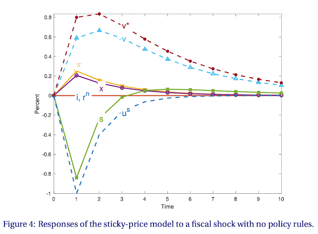
This first response has no policy rules -- the \(\theta\) terms are turned off -- so you can see how the model behaves. The surplus does have an s shaped response, not an AR(1). But it would be darn hard to tell from the AR(1) disturbance \(u^s\). Similarly, the state variable \(v^\ast\) and actual debt \(v\) are similar. The surplus will seem to respond to \(v\) and policy will seem passive if you're not really careful. The initial deficits lead to a rise in debt, which is then slowly paid down by a small string of surpluses.

The fiscal shock leads to a AR(1) pattern of inflation, and as a consequence of the standard Phillips curve an output expansion. With no policy response, interest rates stay put. Now, let's add a monetary and fiscal policy response.

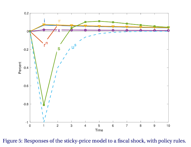
The rise in inflation and output provokes a rise in interest rate. And the initial inflation devalues long term bonds \(r^n\). Together, monetary policy and long term debt substantially reduce the inflationary impact of the fiscal shock and draw it out.  The larger output also gives rise to  larger surpluses, which reduces the size of the fiscal shock to begin with.

Big points: 1) Fiscal theory does not just imply big price level jumps in response to fiscal shocks. Fiscal theory rather naturally here leads to a very long and drawn out inflation in response to a fiscal shock. 2) Endogenous monetary and fiscal policy responses also draw out and buffer the response to a fiscal shock.

Here is the response to a monetary policy shock \(\varepsilon_{m,1}\) holding constant the fiscal policy shock \(\varepsilon_{s,1}\), with no policy rule responses \(\theta=0\). The interest rate and its shock follow an AR(1). Output and inflation decline persistently. Whether true or not in the data, this is the sort of response that is the Holy Grail of monetary theory. At least the model can produce this result.

Surpluses are not constant, because they react to the rise in value of debt that comes from higher real interest rates, represented by the difference between the interest rate and inflation lines. Bond returns follow the expectations hypothesis, mirroring the interest rate with a one period lag, except in the first period. A rise in interest rates leads to a big ex-post decline in bond prices.

Last and most of all, here is the response to monetary policy with policy rules in place.

The interest rate no longer follows its shock. Lower output and inflation bring down the actual interest rate. The monetary policy induced recession now has a deficit too, as the surplus responds to lower output and inflation. Inflation and output still decline in response to the monetary policy shock.

There is a lot more going on here. Real interest rate variation leads to discount rate effects, for example. But I what to whet your appetite to read the paper.

The goal: a really simple baseline fiscal theory of monetary policy model that produces reasonable responses to fiscal and monetary policy. We have drawn out inflation in response to fiscal shocks, not a price level jump; we have lower inflation and output in response to monetary policy not instant Fisherism; and all the AR(1) puzzles are solved. It seems a good place to start. And, for today, to stop.

(Note: this post uses Mathjax to display equations, which is not working perfectly.)

12 May 2020

Bailout redux - Barokong

The greatest financial bailout of all time is underway. It’s 2008 on steroids. Yet where is the outrage? The silence is deafening. Remember the Tea Party and occupy Wall Street? “Never again” they said in 2008. Now everyone just wants the Fed to print more money, faster. (Well, there are some free market economists left. But we're a small voice!)

Maybe the Fed is right that if any bondholder loses money, if bond prices fall, if companies reorganize in bankruptcy, the financial system and the economy will implode. I am not here today to criticize that judgement. But if so, we must ask ourselves how we got to this situation, again, so soon. Once is an expedient. Twice is a habit.  It is clear that going forward any serious shock will be met by bailouts, and the Fed printing reserves to buy vast quantities of any fixed-income asset whose price starts to fall.

Why does the Fed feel the need to jump in? Because once again America is loaded up with debt, because bankruptcy is messy, and because the Fed fears that debt holders losing money will stop the financial system from providing, well, more debt.

This crisis is a huge wealth shock. The income lost during shutdown is simply gone. The question is, who is going to take that loss? Borrowing to keep paying bills, the current solution, posits  that future profits will soak up today's losses. We'll see about that. The CARES act puts future taxpayers squarely on the hook to pay today's bills. But where do those bills go? To creditors -- property owners, bond holders, and so forth. If we're looking around for pots of wealth to absorb today's losses, why are bondholders not chipping in? The biggest wealth transfer in history is underway, from tomorrow's taxpayers to today's bondholders, on the theory that if they lose money the economy falls apart?

OK, but why did America load up with debt again, apparently all "systemically important?" Could the expectation of a bailout any time there is an economy wide shock happens have had something to do with it? Will we do anything when this is over to stop companies from once again loading up with debt -- especially short term debt -- and forcing the Fed's hand again?

Meantime, anyone who hoarded some savings in the hope of profiting from fire sales, in the hope of providing liquidity to "distressed markets" has once again been revealed as a chump. Will we do anything to encourage them? Will lots of debt, private gain, taxpayers take the losses,  be the perpetual character of our financial system.

"You can't worry about moral hazard in a crisis," they said, and they didn't. At least last time there was some recognition of moral hazard, and a promise to clean up the moral hazard with reform. Will there be any such effort this time? Is anyone even thinking about the enormous moral hazard we are creating with these precedents? Will  the financial system perpetually a four-year-old on a bicycle, a parent running closely behind with one hand on the seat? Will the "Powell put" on fixed income grow ever larger? Or will we, this time, finally cure the financial system so it can survive the next shock?

A bailout

Small but symbolic: The federal government just bailed out the airlines -- or more precisely airline stockholders, bondholders, unions, airplane leaseholders and other creditors who would lose in bankruptcy.

"big airlines will receive 70% of the money as grants—which won’t be paid back—and 30% as loans. The cash comes with strings attached: Airlines must give the government warrants amounting to 10% of a given loan’s value that can be swapped for stocks; they cannot lay off staff until September; and they face restrictions on dividends, buybacks and executive compensation."
Oh, and as the article makes clear, this only gets us maybe through the summer. Anyone want to take a bet that planes are full again by September?

The big banks got bailed out in 2008 — or more precisely, the stockholders, bondholders and creditors of the big banks got bailed out.  Never again, they said. Again.

Now, one can make a case that big banks are “systemic,” that if their bondholders lose money the financial system collapses. Just how are airline bondholders “systemic?” What calamity falls if airline bondholders don’t get paid in full?  Just why is a swift pre-packaged bankruptcy not the right answer for airlines? This seems like a great time to renegotiate airplane and gate leases, union contracts (some require the airlines to keep flying empty planes!) fixed-price fuel contracts and more.

If taxpayers have to give airlines cash grants don't we get some reassurance this doesn't have to happen again? Even I would say, no more debt financing. You can see the instinct in "restrictions on dividends, buybacks and executive compensation." Democrats in Congress wanted "stakeholder" board seats, carbon reporting, and more. Why not go full Dodd-Frank on them? Detailed regulation of their financial affairs, stress tests to make sure they can survive the next time? Like banks, the existing airlines might not end up minding so much a return to the 1970s status as regulated utilities. Or, more likely, like GM, we just forget about it, let them load up on debt again, and pretend there won't be a 2030 bailout?

The Fed's big artillery

The real action is at the Fed. The Fed is buying commercial paper, corporate bonds, municipal bonds. The Fed is explicitly propping up asset prices. The Fed is also lending directly to companies. The current guesstimate is $4 trillion, with $2 trillion already accomplished. More is coming.

It started "small"On March 17, the Fed bailed out money market fund investors, buying the “illiquid” assets of those funds so that the funds could continue to pay out dollar for dollar.  Recall that in 2008, the Fed and Treasury bailed out money market fund investors, buying assets to stop a run on money-market funds' promise that you can always cash out at $1. Never again, they said. Fixed dollar promises must be backed by Treasuries, other funds must let asset values float. Again.

On March 17 the Fed also announced it will buy commercial paper.  “Directly from eligible companies.” Yes, the Fed prints reserves to lend directly to companies that can issue A1/P1 commercial paper.

"By eliminating much of the risk that eligible issuers will not be able to repay investors by rolling over their maturing commercial paper obligations, this facility should encourage investors to once again engage in term lending in the commercial paper market. "
Why are companies borrowing long term by rolling over commercial paper? Didn't we learn anything about rolling over short term debt in 2008? Are we going to follow up by putting a stop to that? Why don't companies have more equity financing, on which they can just stop paying dividends?

"Investors" you say, it's not all the Fed. Read carefully. "By eliminating much of the risk..." The Fed props up prices, and removes risk. Then private investors will come in. The markets won't ride that bike without the Fed's hand on the saddle, apparently. Why do we bother to have private markets?

On March 17 the Fed started to lend again to primary dealers. These are the traders, much maligned by the Volcker rule.

The PDCF will offer overnight and term funding with maturities up to 90 days...Credit extended to primary dealers under this facility may be collateralized by a broad range of investment grade debt securities, including commercial paper and municipal bonds, and a broad range of equity securities.
Let's translate. You're the trading desk at, say Goldman Sachs. You want to buy stocks, as you think people are dumping in a hurry. Great, that's what traders are supposed to do: "provide liquidity." But, sadly, you're in the habit of of funding trading activity by borrowing money, short term. And you can't do that right now. So the Fed will now lend you the money to buy stocks, and will take the stocks as collateral! It's almost as if the Fed is buying stocks -- except you get the gains, and if you go under, the Fed gets the stocks! (A friend in the securities industry say nobody is bothering to investigate and price high grade corporates. The Fed is setting the prices.)

Again, the Fed is between a rock and hard place. Yes "balance sheets are constrained." Trading firms don't have enough equity to take on additional risk. The natural buyers at asset fire sales are constrained out of the market. Bail the Fed feels it must. But this is exactly what happened when the Fed first lent to broker/dealers in 2008! Why in the world are we in this position, 12 years after that crisis?

On March 20, the Fed expanded into state and municipal markets. The mechanism is the same: Fed lends to a financial institution, which buys the assets, and then gives the Fed the assets as collateral for the loan. Once again the point is  "enhance the liquidity and functioning of crucial state and municipal money markets."

On March 23, the Fed rolled out real artillery. Ominously,Treasury markets appeared "illiquid," so the Fed has stepped in buying $1.3 trillion in the first month -- more than the Treasury issued.  The Fed is funding Treasury borrowing with newly printed reserves.  The Fed now buys mortgage backed securities.

And now.. corporate bonds. This is well past 2008.

the Primary Market Corporate Credit Facility (PMCCF) for new bond and loan issuance and the Secondary Market Corporate Credit Facility (SMCCF) to provide liquidity for outstanding corporate bonds.
Translation: The Fed will buy new corporate bonds, thus directly lending to corporations. And it will buy  outstanding bonds.

Why would it do that? Well, to "provide liquidity." This is a word that ought to set off BS detectors. Yes, there is such a thing as an "illiquid" market. There is also such a thing as a market whose prices are dropping like a stone. Sell all you want but at 50 cents on the dollar. "I wish I had sold at yesterday's prices" is not illiquidity. You have to pay people a lot to take risk right now. Which is it? Hard to tell. There are ways to tell, of course. For example, illiquid markets have negative price autocorrelation -- a low price today bounces back. I am not aware of the Fed having applied this or any other test. (Research topic suggestion.)

Again, I don't want to criticize, but there sure is a danger of propping up prices under the guise of "illiquidity." The Fed's view that if the Fed takes all risk off the table "liquidity" will reappear is also pretty close to taking risk off the table so prices will rise.

The Fed is already buying new bonds from companies to finance their new expenditures. Propping up prices of existing bonds is a way to let old bondholders cash out at high prices, now before the deluge. Just why can't old bondholders even take mark-to-market losses?

And, if corporate bondholders need to be bailed out in this way, are we going to do anything about it going forward? Do you get to buy junk bonds, high interest municipal debt, and the Fed will let you out if anything bad happens?

Wrap up

OK, I haven't even gotten through March and the Fed is just getting going. Let's wrap up.

The Fed has felt the need to take over essentially all new lending in the economy. The Fed is also propping up most fixed-income prices. The Fed is deliberately removing risk from holding these assets.

Once again, I will be told, "this isn't the time to think about moral hazard." But having done this twice, the first time with huge protest, the second time as if it is perfectly normal, this is the pattern, and the moral hazard is there. The economy will load up on debt, especially short term debt. People will not keep stashes of savings around to provide liquidity or jump on buying opportunities. And the need for bailouts will be larger in the next crisis.

"But the Fed made money in 2008" you may retort. And it has a half chance of making money again. If the recession wraps up in September and these "loans" get paid back, it will do nicely. If the recession goes on a year and all these "loans" go sour, it will not look so pretty.

Yes, in 2008 the Fed and treasury successfully operated the world's largest hedge fund, printing money to buy low-price assets. But is this really the function of the Federal Reserve? Do we want it driving private hedge funds out of the liquidity provision business, by its ability to print rather than borrow money, and by the off-balance-sheet put that the US taxpayer will in the end take losses if this massively leveraged portfolio doesn't work out?

Where is the outrage? Where are the financial economists? Where is the reform plan so we don't do this again? At a minimum, can we say tha  the government could stop subsidizing debt, via tax deduction and regulatory preference for "safe" (ha!) debt as an asset?

Hello out there? In 2008, everyone was writing financial crisis papers. Now everyone is playing amateur epidemiologist.

Finance colleagues, you have a bigger crisis and intervention to study, and a deeper set of regulatory conundrums. Is everyone just too scared of sounding critical of the Fed? Get to work!

The Fed and Treasury's actions are telling us we are on the verge of financial apocalypse. Let's wake up and look at what's coming, especially if it doesn't all get better by September.

Some links

This post continues fromFinancial Pandemic.

I had planned a longer post on the details of many of these programs, but this is long enough.

A great explanation by Robert McCauley in FT. Section heads include  1) Acting as a lender of last resort to securities firms, 2) acting as a lender of last resort to investment funds, 3) acting as a securities dealer of last resort, 4) acting as a securities underwriter of last resort and finally 5) acting as a securities buyer of last resort.

A simple tweet storm by Victoria Guida

Via the indefatigable Torsten Slok,

Financial Policy During the COVID-19 Crisis MIT opeds on financial affairs

A great list of policy trackers.

Financing Firms in Hibernation During the COVID-19 Pandemic

The YaleFinancial Stability Tracker and especially theFinance Response Tracker are very useful list of what's going on.

Fed Intervention in the To-Be-Announced Market for Mortgage-Backed Securities

by Bruce Mizrach and Christopher J. Neely is a very nice description of what's going on there

The United States as a Global Financial Intermediary and Insurer by Alexander Monge-Naranjo. More contingent liabilities waiting for Uncle Sam bailouts.

A data set of international fiscal responses

English

Anies Baswedan

Tekno